2.2 Basic Concepts - Inverse Trigonometric Functions - Class 12 Mathematics
2.2 Basic Concepts
Screen Readable NCERT Class 12 Mathematics Textbook for blind and low vision students prepared by Dr T K Bansal.
In Class 11, we have studied trigonometric functions, which are defined as follows:
sine function, i.e., \(\sin\ :\ R\ →\ [−1,\ 1]\)
cosine function, i.e., \(\cos\ :\ R\ →\ [−1, 1]\)
tangent function, i.e., \(\tan\ :\ R\ −\ \{x\ :\ x\ =\ (2n+1)\frac{π}{2},\ n∈Z\}\ →\ R\)
cotangent function, i.e., \(\cot\ :\ R\ −\ \{x\ :\ x\ =\ nπ,\ n∈Z\}\ →\ R\)
secant function, i.e., \(\sec\ :\ R\ −\ \{x\ :\ x=(2n+1) \frac{π}{2},\ n∈Z\}\ →\ R\ −\ (−1,\ 1)\)
cosecant function, i.e., \(\csc\ :\ R\ −\ \{x\ :\ x=nπ,\ n∈Z\}\ →\ R\ −\ (−1,\ 1)\)
We have also learnt in Chapter 1 that if
f : X → Y, such that f(x) = y,
is one-one and onto, then we can define a unique function
g : Y → X, such that g(y) = x,
where x ∈ X and y = f(x), y ∈ Y.
Here, the domain of g = range of f and the range of g = domain of f.
The function g is called the inverse of f and is denoted by f^−1.
Further, g is also one-one and onto and inverse of g is f.
Thus, g^−1 = (f^−1)^−1 = f.
We also have
(f^−1 o f)(x) = f^−1 (f(x)) = f^−1(y) = x
and
(f o f^−1) (y) = f (f^−1(y)) = f (x) = y
Defining \(\sin^{−1} x\)
Since the domain of sine function is the set of all real numbers and range is the closed interval [−1, 1], as such, its inverse can not be defined.
However, if we restrict its domain to \([\frac{−π}{2},\ \frac{π}{2}],\) then it becomes one-one and onto with range [− 1, 1].
Actually, sine function restricted to any of the intervals,
\([\frac{−3π}{2},\ \frac{−π}{2}],\)
\([\frac{−π}{2},\ \frac{π}{2}],\)
\([\frac{π}{2},\ \frac{3π}{2}]\)
etc, is one-one and its range is [ −1, 1]. We can, therefore, define the inverse of sine function in each of these intervals.
We denote the inverse of sine function by sin^−1 (arc sine function). Thus, sin^−1 is a function whose domain is [ − 1, 1] and range could be any of the intervals [ −3π/2, −π/2], [ −π/2, π/2] or [π/2, 3π/2], and so on.
Corresponding to each such interval, we get a branch of the function sin^−1. The branch with range \([\frac{−π}{2},\ \frac{π}{2}]\) is called the principal value branch, whereas other intervals as range give different branches of sin^−1.
When we refer to the function sin^−1, we take it as the function whose domain is [ −1, 1], and whose range is [ −π/2, π/2].
We write
\[\sin^{−1}\ :\ [−1,\ 1]\ →\ [\frac{−π}{2},\ \frac{π}{2}]\]
From the definition of the inverse functions, it follows that
sin (sin^−1 x) = x if −1 ≤ x ≤ 1 and
sin^−1 (sin x) = x if −π/2 ≤ x ≤ π/2.
In other words, if y = sin^−1 x, then sin y = x.
Remarks:
(i) We know from Chapter 1, that if y = f (x) is an invertible function, then x = f^−1 (y). Thus, the graph of sin^−1 function can be obtained from the graph of original function by interchanging x and y axes, i.e., if (a, b) is a point on the graph of sine function, then (b, a) becomes the corresponding point on the graph of inverse of sine function. Thus, the graph of the function y = sin^−1 x can be obtained from the graph of y = sin x by interchanging x and y axes. The graphs of y = sin x and y = sin^−1 x are as given in Figure 2.1(i), and Figure2.1(ii), (Figure 2.1iii). The dark portion of the graph of y = sin^−1 x represent the principal value branch.
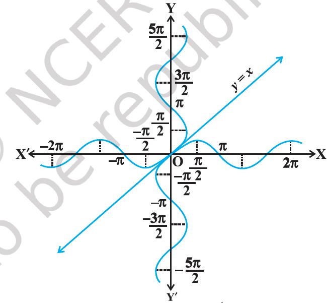
(ii) It can be shown that the graph of an inverse function can be obtained from the corresponding graph of original function as a mirror image (i.e., reflection) along the line y = x. This can be visualized by looking at the graphs of y = sin x and y = sin^−1 x as given in the same axes (Figure 2.1 (iii)).
Figure 2.1 (i) y = sin x
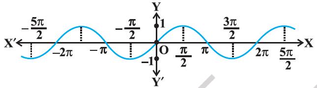
Figure 2.1 (ii)y = sin^−1 x
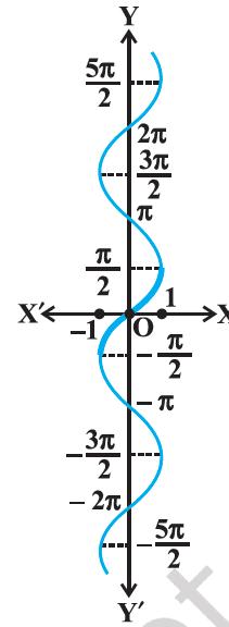
Figure 2.1 (iii) y = sin x and y = sin^−1 x
Defining \(\cos^{−1}x\)
Like sine function, the cosine function is a function whose domain is the set of all real numbers and range is the set [−1, 1].
If we restrict the domain of cosine function to [0, π], then it becomes one-one and onto with range [ −1, 1].
Actually, cosine function restricted to any of the intervals
[−π, 0],
[0, π],
[π, 2π],
etc, is bijective with range as [ −1, 1].
We can, therefore, define the inverse of cosine function in each of these intervals. We denote the inverse of the cosine function by cos^−1 (arc cosine function). Thus, cos^−1 is a function whose domain is [ −1, 1] and range could be any of the intervals [ −π, 0], [0, π], [π, 2π] etc.
Corresponding to each such interval, we get a branch of the function cos^−1.
The branch with range [0, π] is called the principal value branch of the function cos^−1.
We write
\[\cos^{−1}\ :\ [−1,\ 1]\ →\ [0,\ π].\]
The graph of the function given by y = cos^−1 x can be drawn in the same way as discussed about the graph of y = sin^−1 x. The graphs of y = cos x and y = cos^−1x are given in Figure 2.2 (i) and Figure 2.2(ii).
Figure 2.2 (i) y = cos x
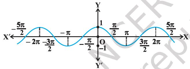
Figure 2.2 (ii) y = cos^−1x
Defining \(\csc^{−1}x\) and \(\sec^{−1}x\)
Let us now discuss cosec^−1 x and sec^−1 x as follows:
Since,
\[\csc x\ =\ \frac{1}{\sin x},\]
the domain of the cosec function is the set {x : x ∈ R and x ≠ nπ, n ∈ Z},
and the range is the set {y : y ∈ R, y ≥ 1 or y ≤ −1} i.e., the set R − ( −1, 1).
It means that y = cosec x assumes all real values except −1 < y < 1 and is not defined for integral multiples of π.
If we restrict the domain of cosec function to [−π/2, π/2] − {0}, then it is one to one and onto with its range as the set
R − ( − 1, 1).
Actually, cosec function, restricted to any of the intervals
[ −3π/2, −π/2] − {−π},
[−π/2, π/2] − {0},
[π/2, 3π/2] − {π} etc,
is bijective and its range is the set of all real numbers R − (−1, 1).
Thus cosec^−1 can be defined as a function whose domain is R − (−1, 1) and range could be any of the intervals
[−3π/2, −π/2] − {−π},
[−π/2, π/2] − {0},
[π/2, 3π/2] − {π} etc.
The function corresponding to the range [−π/2, π/2] − {0} is called the principal value branch of cosec^−1. We thus have principal branch as
\[\csc^{−1}\ :\ R\ −\ (−1,\ 1)\ →\ [\frac{−π}{2},\ \frac{π}{2}]\ −\ {0}\]
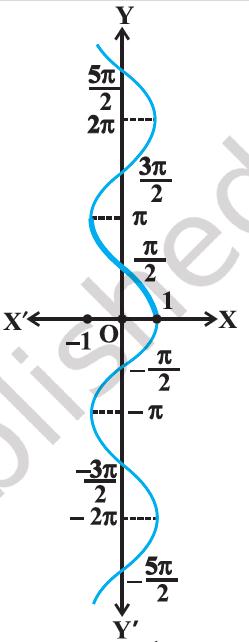
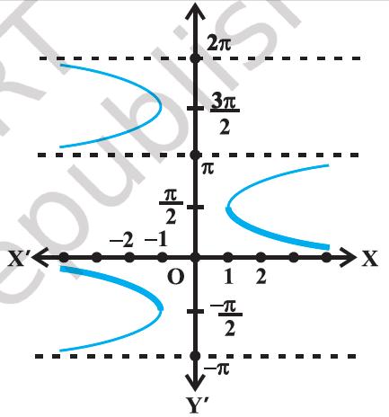
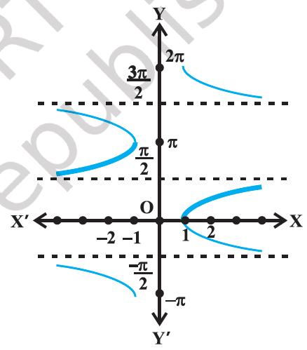
The graphs of y = cosec x and y = cosec^−1 x are given in Figure 2.3(i), Figure 2.3(ii).
Figure 2.3(i) y = cosec x
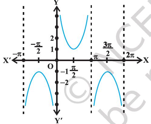
Figure 2.3(ii) y = cosec^−1 x
Also, since \(\sec x\ =\ \frac{1}{\cos x},\)
the domain of y = sec x is the set R − {x : x = (2n + 1) (π/2), n ∈ Z}
and the range is the set R − (−1, 1).
It means that sec (secant function) assumes all real values except −1 < y < 1 and is not defined for odd multiples of π/2.
If we restrict the domain of secant function to [0, π] − {π/2}, then it is one-one and onto with its range as the set R − ( −1, 1).
Actually, secant function restricted to any of the intervals
[ −π, 0] − { −π/2},
[0, π] − {π/2},
[π, 2π] − {3π/2} etc.,
is bijective and its range is R − {−1, 1}.
Thus sec^−1 can be defined as a function whose domain is R − (−1, 1) and range could be any of the intervals
[ −π, 0] − { −π/2},
[0, π] − {π/2},
[π, 2π] − {3π/2} etc.
Corresponding to each of these intervals, we get different branches of the function sec^−1.
The branch with range [0, π] − {π/2} is called the principal value branch of the function sec^−1.
We thus have
\[\sec^{−1}\ :\ R\ −\ (−1,\ 1)\ →\ [0,\ π]\ −\ \{\frac{π}{2}\}\]
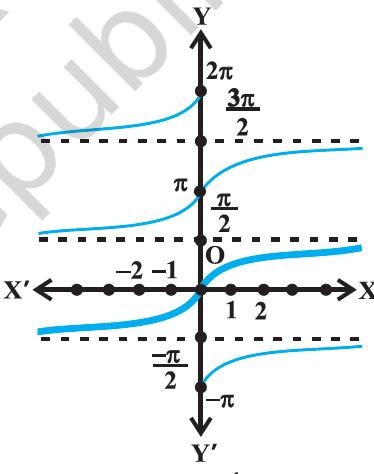
The graphs of the functions y = sec x and y = sec^−1 (x) are given in Figure 2.4(i), and Figure 2.4(ii).
Figure 2.4 (i) y = sec x
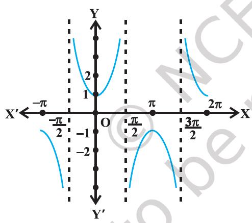
Figure 2.4 (ii) y = sec^−1( x)
Defining \(\tan^{−1}x\) and \(\cot^{−1}x\)
We know that the domain of the tan function (tangent function) is the set {x : x ∈ R and x ≠ (2n +1) π/2, n ∈ Z}
and the range is R.
It means that tan function is not defined for odd multiples of π/2, moreover, tan x is not a one-one function.
If we restrict the domain of tangent function to ( −π/2, π/2), then it is one-one and onto with its range as R.
Actually, tangent function restricted to any of the intervals
( −3π/2, −π/2 ),
( −π/2, π/2 ),
( π/2, 3π/2 ) etc.,
is bijective and its range is R.
Thus tan^−1 can be defined as a function whose domain is R and range could be any of the intervals
(−3π/2, −π/2),
(−π/2, π/2),
(π/2, 3π/2) and so on.
These intervals give different branches of the function tan^−1.
The branch with range ( −π/2, π/2) is called the principal value branch of the function tan^−1.
We thus have
\[\tan^{−1}\ :\ R\ →\ (\frac{−π}{2},\ \frac{π}{2})\]
The graphs of the function y = tan x and y = tan^−1x are given in Figure 2.5(i), and Figure 2.5(ii).
Figure 2.5 (i) y = tan x
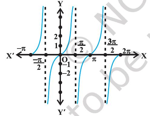
Figure 2.5 (ii) y = tan^−1(x)
We know that the domain of the cot function (cotangent function) is the set {x : x ∈ R and x ≠ nπ, n ∈ Z},
and the range is R.
It means that cotangent function is not defined for integral multiples of π, and it is not a one-one function.
If we restrict the domain of cotangent function to (0, π), then it is bijective and with its range as R.
In fact, cotangent function restricted to any of the intervals
( −π, 0),
(0, π),
(π, 2π) etc.,
is bijective and its range is R.
Thus cot^−1 can be defined as a function whose domain is the R and range as any of the intervals
( −π, 0),
(0, π),
(π, 2π) etc.
These intervals give different branches of the function cot^−1.
The function with range (0, π) is called the principal value branch of the function cot^−1.
We thus have
\[\cot^{−1}\ :\ R\ →\ (0,\ π)\]
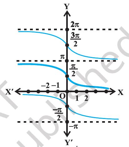
The graphs of y = cot x and y = cot^−1x are given in Figure 2.6(i), and Figure 2.6(ii).
Figure 2.6 (i) y = cot x
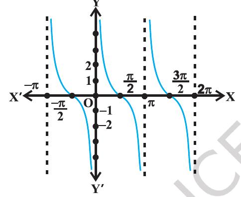
Figure 2.6 (ii) y = cot−1 (x)
The following table gives the inverse trigonometric function (principal value branches) along with their domains and ranges.
| sin^−1 : [−1, 1] → [−π/2, π/2] |
| cos^−1 : [−1, 1] → [0, π] |
| cosec^−1 : R − (−1, 1) → [−π/2, π/2] − {0} |
| sec^−1 : R − (−1, 1) → [0, π] − {π/2} |
| tan^−1 : R → (−π/2, π/2) |
| cot^−1 : R → (0, π) |
Note carefully
1.
sin^−1 (x) should not be confused with (sin x)^−1. In fact (sin x)^−1 = 1/sin x and similarly for other trigonometric functions.
2.
Whenever no branch of an inverse trigonometric functions is mentioned, we mean the principal value branch of that function.
3.
The value of an inverse trigonometric functions which lies in the range of principal branch is called the principal value of that inverse trigonometric functions.
Let us now consider some examples:
Example 1
Find the principal value of \(\sin^{−1} \frac{1}{√2}\)
Solution:
Let sin^−1 (1/√2) = y.
Then, sin y = 1/√2.
We know that the range of the principal value branch of sin^−1 is [−π/2, π/2],
and sin(π/4) = 1/√2.
Therefore, principal value of sin^−1(1/√2) is π/4
Example 2
Find the principal value of \(\cot^{−1} \frac{−1}{√3}\)
Solution:
Let cot^−1(−1/√3) = y.
Then,cot y = −1/√3 = − cot(π/3)
= cot(π − π/3)
= cot (2π/3)
We know that the range of principal value branch of cot^−1 is (0, π) and cot (2π/3)
= −1/√3. Hence, principal value of cot^−1(−1/√3) is 2π/3.
EXERCISE 2.1
Find the principal values of the following:
Question 1
\[\sin^{−1}(\frac{−1}{2})\]
Answer 1
−π/6
Question 2
\[\cos^{−1}(\frac{√3}{2})\]
Answer 2
π /6
Question 3
\[\csc^{−1}(2)\]
Answer 3
π /6
Question 4
\[\tan^{−1}(−√3)\]
Answer 4
−π/3
Question 5
\[\cos^{−1}(\frac{−1}{2})\]
Answer 5
(2π)/6
Question 6
\[\tan^{−1}(−1)\]
Answer 6
−π/4
Question 7
\[\sec^{−1}(\frac{2}{√3})\]
Answer 7
π/6
Question 8
\[\cot^{−1} (√3)\]
Answer 8
π /6
Question 9
\[\cos^{−1}(\frac{−1}{√2})\]
Answer 9
3π/4
Question 10
\[\csc^{−1} (−√2)\]
Answer 10
−π/4
Find the values of the following:
Question 11
\[\tan^{−1}(1)\ +\ \cos^{−1} (\frac{−1}{2})\ +\ \sin^{−1} (\frac{−1}{2})\]
Answer 11
3π/4
Question 12
\[\cos^{−1} (\frac{1}{2})\ +\ 2 \sin^{−1} (\frac{1}{2})\]
Answer 12
2π/3
Question 13
If \(\sin^{−1} (x)\ =\ y,\) then
(A) 0 ≤ y ≤ π
(B) −π/2 ≤ y ≤ π/2
(C) 0 < y < π
(D) −π/2 < y < π/2
Answer 13
B
Question 14
\[\tan^{−1} (√3)\ −\ \sec^{−1} (−2) =\]
(A) π
(B) − π/3
(C) π/3
(D) 2π/3
Answer 14
B